Idempotent Backward Slice
Have you ever wondered what programmers ask themselves when they need to fix a bug in a program? They need to understand how the program’s variables, functions, and data structures interact with each other. However, a program can be very large, and one doesn’t need to cover all instructions to fix a specific issue. Therefore, they can limit the scope of the search by selecting just a subset of instructions used to compute a given value at a program point. This subset of instructions is called a program slice [8], and it is an executable program that, given an input value, will always produce an output at the end of its execution.
Following the problem statement, we provide definitions to contextualize our discussion. Then, we present an algorithm to compute idempotent slices backwardly. Additionally, we demonstrate how to perform the same task more efficiently using programs in SSA form. Finally, we conclude this study in the corresponding section.
Note: this post references a video I produced as part of a series on compiler research topics, available on the Compilers Laboratory’s YouTube channel.
Problem Statement
Given a slice criterion, the goal is to compute all data and control dependencies backwardly in the CFG of a program. A slice criterion typically consists of a specific program point and a set of variables of interest at that point.
By analyzing the program’s CFG, we can identify all instructions that directly or indirectly affect the values of these variables at the given program point. This involves tracing both data dependencies, which capture how data values are propagated through the program, and control dependencies, which capture how the execution flow of the program is influenced by conditional statements.
The result is a backward slice, a subset of the program that includes only the relevant instructions needed to understand the behavior of the variables at the specified program point. Additionally, the new slice must be idempotent [6], meaning that given the same input, the program must consistently return the same value.
Definitions
In this section we define some terms that will be explored throughout this article.
Control Flow Graph
A program is represented as a control flow graph (CFG):
- A digraph \(G = (N, E)\) consists of:
- \(N\): set of program statements (nodes).
- \(E\): directed edges representing control flow between statements.
- A control flow graph \((N, E, n_0)\) is a digraph where \(n_0\) is the entry node.
- Start: \(n_0\), or a special node that can reach every other node, but no other node can reach it [5].
- A hammock graph \((N, E, n_0, n_e)\) [3] is a control flow graph with a unique exit node \(n_e\).
- End: \(n_e\), or a special node that is reachable from every other node, but does not reach any other node [5].
Def-use Chain
Let \(V\) be the set of variables in a program \(P\). For each statement \(n\):
- \(\text{USE}(n)\): set of variables used at \(n\).
- \(\text{DEF}(n)\): set of variables modified at \(n\).
State Trajectory
A state trajectory of length \(k\) is a sequence: \((n_1, s_1), (n_2, s_2), ..., (n_k, s_k)\) where each \(n_i\) is a statement and each \(s_i\) is a mapping of variables to values.
Slicing Criterion
A slicing criterion \(C = (i, V)\) specifies:
- \(i\): a statement index where slicing occurs.
- \(V\): a subset of variables observed at \(i\).
Projection Function
A projection function extracts only relevant information from a state trajectory: \(\text{Proj}_{(i,V)}(n, s) = \begin{cases} (n, s \mid V), & \text{if } n = i \\ X, & \text{otherwise} \end{cases}\)
where \(s \mid V\) restricts \(s\) to the variables in \(V\).
For a trajectory \(T\), we apply: \(\text{Proj}_{(i,V)}(T) = \text{Proj}_{(i,V)}(t_1) ... \text{Proj}_{(i,V)}(t_n).\)
Program Slice
A slice \(S\) of a program \(P\) satisfies:
- \(S\) is obtained by deleting zero or more statements from \(P\).
- \(S\) produces the same projection as \(P\) for all inputs where \(P\) terminates.
Dataflow Analysis
In this analysis, we are interested on gathering information about what may happen in a program at run time, without running it [1]. This analysis will be a conservative approximation of its behaviour and flow sensitive. A flow sensitive analysis considers the order in which variables are defined and used in a program [5].
Static Single-Assignment Form (SSA)
The static single-assignment (SSA) form is a program representation in which each variable is assigned exactly once [2]. Therefore, the Single Information Property holds when the information associated with a variable \(v\) during dataflow analysis remains invariant at every program point where it is alive [4]. This property simplifies dataflow analysis and facilitates reasoning about the behavior of a program.
In SSA form:
- Each variable is assigned a unique name whenever it is defined.
- If a variable is defined in multiple control flow paths, a special \(\phi\)-function is introduced to merge the values from these paths.
Example
Consider the following code snippet:
1
2
3
4
5
6
if (x > 0) {
  y = 1;
} else {
  y = 2;
}
z = y + 3;
In SSA form, the code is transformed as follows:
1
2
3
4
5
6
7
if (x > 0) {
  y1 = 1;
} else {
  y2 = 2;
}
y3 = phi(y1, y2);
z1 = y3 + 3;
Here, the \(\phi\)-function combines the values of y1 and y2 based on the control flow.
Program Dependency Graph
Following [3], we define a program dependency graph (PDG) in the context of SSA form. A PDG is a directed graph \(G = (V, E)\), where \(V\) represents the set of vertices, with one vertex corresponding to each variable in the program. The set \(E\) consists of directed edges, where an edge \((u, v) \in E\) exists if and only if \(v\) appears on the left-hand side of an instruction in which \(u\) appears on the right-hand side. An edge can be either solid or dotted: the former represents explicit dependencies, while the latter represents implicit dependencies.
Dominance
Dominance relationships between the nodes of a Control Flow Graph (CFG) are defined below, following [5]:
- Dominance: A node \(m\) dominates \(n\) if every path from the Start node to \(n\) passes through \(m\).
- Immediate Dominance: A node \(m\) is the immediate dominator of \(n\) if \(m\) dominates \(n\), and for any other node \(p\) that also dominates \(n\), \(p \neq m\) implies that \(m\) dominates \(p\).
- Post-Dominance: A node \(m\) post-dominates \(n\) if every path from \(n\) to the Exit node passes through \(m\).
- Immediate Post-Dominance: A node \(m\) is the immediate post-dominator of \(n\) if it is the dual of immediate dominance, meaning \(m\) post-dominates \(n\), and for any other node \(p\) that post-dominates \(n\), \(p \neq m\) implies that \(m\) post-dominates \(p\).
Dominator Tree
Knowing that the immediate dominator and the immediate post-dominator of any basic block in a CFG are unique [1], we define a dominance tree and a post-dominance tree.
Weiser’s Algorithm
Although Weiser [8] proofs that there is no algorithm to compute statement-minimal slices, it is possible to use data and control flow analysis to approximate the computation of program slices.
Step 1: Compute Directly Relevant Variables
Define \(R_C(n)\), the set of relevant variables at statement \(n\): \(R_C(n) = \begin{cases} V, & \text{if } n = i \\ \{ v \mid v \in \text{USE}(n) \text{ and } w \in \text{DEF}(n) \cap R_C(m) \}, & \text{if } m \text{ is a successor of } n \end{cases}\)
This ensures that variables affecting \(V\) at \(i\) are traced back through the program.
Step 2: Identify Control Dependencies
A statement \(b\) influences a statement \(s\) if it controls whether \(s\) executes. Define INFL as: \(\text{INFL}(b) = \{ n \mid n \text{ is on a path from } b \text{ to its nearest post dominator} \}.\)
All statements affecting any \(n \in S_C\) are included in the slice.
Step 3: Construct the Slice
The final slice \(S_C\) consists of all statements where: \(R_C(n+1) \cap \text{DEF}(n) \neq \emptyset.\)
Efficient Algorithm for Sparse Slicing
Weiser’s algorithm performs a dense analysis of a program by associating information with pairs consisting of variables and program points. However, his approach to identifying data and control dependencies can be improved by utilizing more efficient data structures, rather than computing consecutive sets of transitively relevant statements [7]. To address this, we present an algorithm that computes program slices using a sparse analysis, which handles data and control dependencies more efficiently [5].
Dense vs. Sparse Analysis
A dense analysis computes data and control dependencies by associating information with pairs of variables and program points. Each program point represents a region between two instructions in a Control Flow Graph (CFG). This approach has a worst-case complexity of \(\mathcal{O}(V^2)\), where \(V\) is the number of variables. However, by leveraging the SSA form, we can reduce this quadratic complexity to \(\mathcal{O}(V)\).
To achieve this, the program must first be transformed into Static Single Assignment (SSA) form. In SSA form, each variable is assigned exactly once, and all the information we need to track is bound to the variable’s name. This transformation enables a more efficient computation of dependencies.
Consider the C code in Program 1. It’s SSA from is presented in a CFG by Figure 1.
1
2
3
4
5
6
7
8
9
10
a = 0;
b = 0;
do {
    while (b < 13) {
        b = b + 1;
        x = x + a * b;
    }
    a = a + 1;
} while (a < 17);
use(b);
Program 1: Example C program.
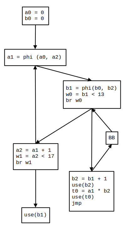
Figure 1: The program’s Control Flow Graph (CFG) in SSA form.
Computing Dependencies with PDG and Dominator Tree
To compute data and control dependencies between variables, we use the Program Dependency Graph (PDG) and the Dominator Tree. The PDG represents dependencies between program variables, while the Dominator Tree captures dominance relationships between nodes in the CFG.
Building the PDG: After selecting a slice criterion (e.g., a variable or program point of interest), a Breadth-First Search (BFS) is performed over the PDG to identify all relevant dependencies. The PDG is constructed by analyzing the program’s data flow and control flow, linking variables and instructions based on their dependencies.
Building the Dominator Tree: To construct the Dominator Tree, we perform a dominance analysis over the CFG. This analysis identifies the dominance relationships between nodes, where a node \(m\) dominates another node \(n\) if every path from the Start node to \(n\) passes through \(m\). The resulting tree maps each node in the CFG to its immediate dominator, enabling efficient traversal and dependency analysis.
The program’s Dominator Tree and Program Dependency Graph (PDG) are shown in Figures 2, and 3, respectively. These structures are used to compute an idempotent backward slice based on the slice criterion use(b2) (Figure 4). The resulting slice is shown in Figure 4(c).
Influence Region
The influence region of a block \(B\) is the set of blocks dominated by \(B\) but not post-dominated by it. This region determines which variables are affected by a predicate.
Algorithm Overview
- Input: A program in SSA form, represented as a dominance tree.
- Output: A slice containing only relevant instructions.
- Steps:
- Traverse the dominance tree to identify the influence region of each predicate.
- Link predicates to variables defined within their influence region.
- Use the PDG to compute transitive dependencies efficiently.
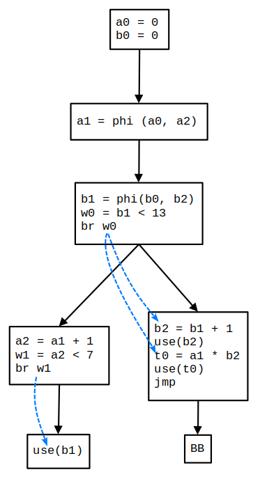
Figure 2: The program’s Dominator Tree.
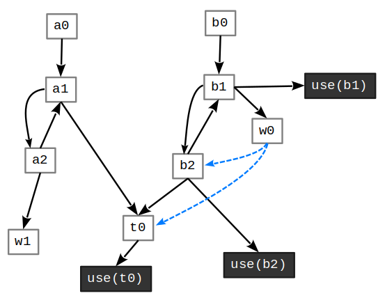
Figure 3: The program’s Program Dependency Graph (PDG).
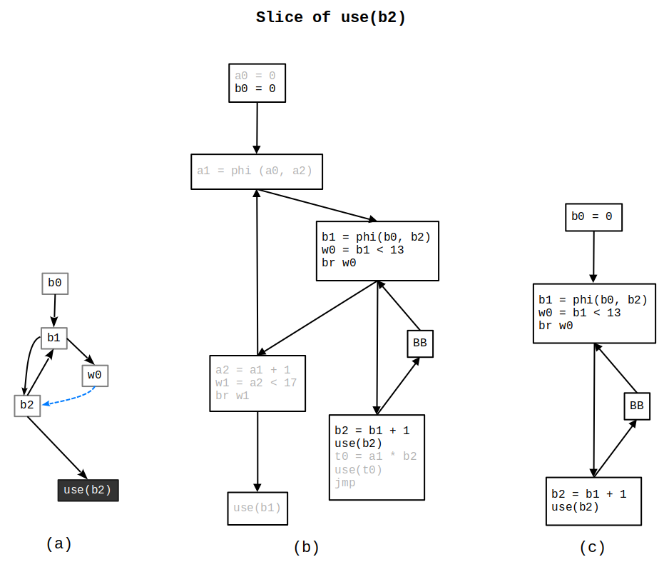
Figure 4: (a) PDG fragment; (b) CFG fragment; (c) Outlined function.
The algorithm presented here improves upon Weiser’s dense analysis by transforming the program into SSA form. This transformation allows us to perform a sparse analysis, significantly reducing the complexity of computing program slices from \(\mathcal{O}(V^2)\) to \(\mathcal{O}(V)\).
By utilizing the Program Dependency Graph (PDG) and Dominator Tree, we efficiently compute both data and control dependencies, enabling precise and efficient slicing. The example demonstrates how the algorithm operates on a real program, showcasing its ability to compute an idempotent backward slice with improved performance and accuracy.
Conclusion
In this study, we examined idempotent backward slicing—a precise and effective technique for program analysis and debugging. By formalizing key definitions and outlining the associated algorithm, we provided a structured foundation for understanding and applying this method to isolate program instructions that influence specific variables.
Idempotent backward slices ensure reliability and repeatability in analysis, making them a valuable tool for developers and researchers alike. This work lays the groundwork for further exploration of slicing techniques across various software engineering domains. For a practical implementation within an LLVM pass, see project Daedalus.
We encourage readers to consult the cited references for deeper insights into the theory and evolution of program slicing, as ongoing research continues to advance its effectiveness in analyzing and debugging complex systems.
References
[1] Appel, Andrew W., and Maia Ginsburg. Modern Compiler Implementation in C. New, Expanded textbook, Cambridge Univ. Press, 2004.
[2] Cytron, Ron, et al. Efficiently Computing Static Single Assignment Form and the Control Dependence Graph. ACM Transactions on Programming Languages and Systems, vol. 13, no. 4, pp. 451–90. 1991.
[3] Ferrante, Jeanne, et al. The Program Dependence Graph and Its Use in Optimization. ACM Transactions on Programming Languages and Systems, vol. 9, no. 3, pp. 319–349. 1987.
[4] Rastello, Fabrice, and Florent Bouchez Tichadou, editors. SSA-Based Compiler Design. Springer International Publishing, 2022.
[5] Rodrigues, Bruno, et al. Sparse Representation of Implicit Flows with Applications to Side-Channel Detection. Proceedings of the 25th International Conference on Compiler Construction, ACM, pp. 110–20. 2016.
[6] Rosen, Kenneth H., and Kamala Krithivasan. Discrete Mathematics and Its Applications. 7. ed., Global ed, McGraw-Hill. 2013.
[7] Tip, Frank. A Survey of Program Slicing Techniques. CWI (Centre for Mathematics and Computer Science), NLD. 1994.
[8] Weiser, Mark. Program Slicing. IEEE Transactions on Software Engineering, vol. SE-10, no. 4, pp. 352–57. 1984.